1. Simulating a Waveguide in 2D
Before delving into the details of how to use EMopt to optimize electromagnetic structures, it is a good idea to first familiarize yourself with how setup and run simulations using the tools provided (which will ultimately provide the foundation for optimizations). The following tutorial will demonstrate how to simulate a simple waveguide structure using EMopt’s 2D Maxwell solver. Furthermore, it will help you familiarize yourself with EMopt’s approach to solving electromagnetic problems.
Note
Example Code The code associated with this tutorial can be found in examples/simple_waveguide/simple_waveguide.py
Note
Running the code
In order to run code written on top of EMopt, you are encouraged to take advantage of MPI for parallelism. EMopt is built on top of MPI from the ground up in order to accelerate its execution. In order to run this example using MPI on, for example, 4 cores, you would run the command:
$ mpirun -n 4 python simple_waveguide.py
1.1. Importing the Required Libraries
In order to use EMopt, the first thing we must do is import the EMopt module.
For access to most components of EMopt, we will simply import the top-level
module emopt:
import emopt
As we fill find out in just a moment, all submodules, classes and functions can
be called using emopt.X.Y where X is the submodule and Y is the class or
function. In this example, we will explicitly import one addition EMopt
variable which will come in handy later on in the tutorial:
from emopt.misc import NOT_PARALLEL
Finally, almost all mathematical operations will make use of the numpy library.
As such, we need to import numpy:
import numpy as np
At this point, we are ready to start using EMopt!
1.2. Setting up the Simulation Domain
The first step in setting up a simulation is to define the dimensions of the simulation domain, the resolution of the simulation grid, and the wavelength of the source excitation. We do this by defining corresponding variables and then instantiating an FDFD object, supplying those variables as parameters:
W = 10.0
H = 7.0
dx = 0.02
dy = 0.02
wlen = 1.55
sim = emopt.fdfd.FDFD_TE(W, H, dx, dy, wlen)
In this example, we will make the simulation 10 μm wide by 7 μm tall. Notice
that we wrote this simply as 10.0 and 7.0, respectively and not, for example,
10e-6 and 7e-6 (i.e. in metric). This is
because EMopt solves non-dimensionalized equations. In the case of length
quantities, everything is normalized with respect to the wavelength. This means
that if we want the wavelength to be 1.55 μm and we want to express all other
lengths in units of μm, we simply set wavelength = 1.55 (as we did above).
As long as we are consistent with these units everything works out.
The simulation resolution, meanwhile, is set by defining a spatial
discretization size (or grid cell size) along the x and y. In this example,
we choose these dimensions, given by dx and dy, to be 20 nm. Note that
currently, EMopt only supports uniform rectangular grids (which should be
sufficient or even desirable in most cases).
Finally, in the last line above, we instantiate an FDFD_TE object.
FDFD stands for Finite Difference Frequency Domain and refers
to the method we will use to solve Maxwell’s Equations in 2D. TE, meanwhile,
refers to “transverse electric” and idicates that we will be solving for the
fields \(E_z\), \(H_x\), and \(H_y\). Depending on the problem we
wish to solve, EMopt also provides the FDFD_TM class for 2D TM
simulations.
One thing that is important to be aware of is that you are not required to
select simulation widths which are exactly divisible by the grid spacing. In
the case that W/dx and/or H/dy are not integers, EMopt will automatically
modify “snap” the simulation dimensions to the nearest grid cell. As such, it
is generally a good idea to update the W and H variables after
instantiating the FDFD object. Furthermore, the FDFD object also exposes the
number of grid cells along the x and y directions. To access these
variables:
W = sim.W
H = sim.H
N = sim.N
M = sim.M
Here, N is the number of grid cells along the x direction and M is
the number of grid cells along the y directions (this matches matrix/array
index notation).
1.3. Defining the Structure and Materials
Our ultimate goal is to simulate a 2D waveguide which is excited by a dipole
source. As such, we need to define the waveguide, which is ultimately just a
particular distribution of permittivity and permeability. EMopt provides a few
ways of defining material distributions, however the most common approach is
through the use of the StructuredMaterial2D and
ConstantMaterial2D classes.
In order to define a simple waveguide, we will create a rectangle with the desired position and dimensions. We will then assign this rectangle a permittivity value and a layer. Lower number layers will appear on top of layers with higher numbers (in other words, lower number = higher priority). Just as with the waveguide, we will define a background/cladding material. The process is as follows:
# Materials
n0 = 1.0
n1 = 3.0

# set a background permittivity of 1
eps_background = emopt.grid.Rectangle(W/2, H/2, 2*W, H)
eps_background.layer = 2
eps_background.material_value = n0**2

# Create a high index waveguide through the center of the simulation
h_wg = 0.5
waveguide = emopt.grid.Rectangle(W/2, H/2, 2*W, h_wg)
waveguide.layer = 1
waveguide.material_value = n1**2
In EMopt, emopt.grid.Rectangles belong to a broader class of elements called
MaterialPrimitives. A MaterialPrimitive is a shape which
can be combined with other shapes in order to form more complex structures. In
order to combine shapes together into complex structures, we use a
emopt.grid.StructuredMaterial2D which is a container for
MaterialPrimitives that facilitates the generation of material
distributions based on collections of MaterialPrimitives.
In order to define the permittivity distribution, all we need to do is create a
emopt.grid.StructuredMaterial2D which contains the cladding and waveguide
rectangles:
eps = emopt.grid.StructuredMaterial2D(W, H, dx, dy)
eps.add_primitive(waveguide)
eps.add_primitive(eps_background)
At this point, we have defined a permittivity distribution, which we can
generate using StructuredMaterial2D.get_values() and which is depicted
below.
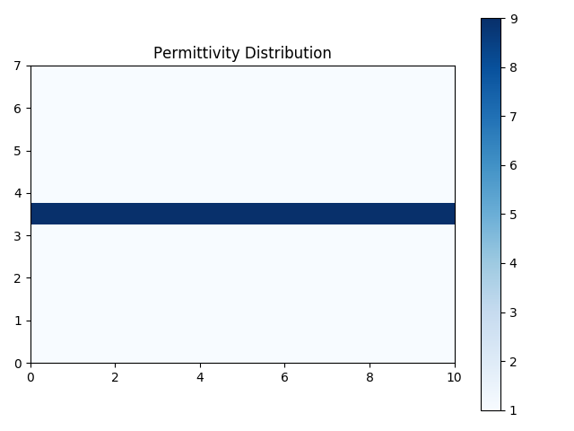
Permittivity distribution for a simple waveguide.
Note
Complex Material Values
EMopt supports both real and complex material values in 2D. To define a
complex material, we simply write material_value = a + 1j*b where
a and b are numbers.
The permeability distribution can be defined in an identical manner. At optical
frequencies, in many cases the permeability is assumed to be uniformly equal to
1.0. We make this same assumption in this tutorial. EMopt provides a simple
way to define uniform constant material distributions using the
emopt.grid.ConstantMaterial2D class:
mu = emopt.grid.ConstantMaterial2D(1.0)
With permittivity and permeability distributions defined, our last step in defining the simulated structure is to actually set the material distributions in our simulation (which is encapsulated by the FDFD object we created earlier). To do this, we simply write:
sim.set_materials(eps, mu)
With this, we have finished defining the structure that we will simulate.
1.4. Defining the Sources
The final missing ingredient in setting up our simulation is the source. Sources consist of some arrangement of electric and magnetic dipoles (small oscillating currents). EMopt provides two ways of defining the current sources in a 2D simulation. First, you can explicitly define arrays which specify the distribution of the complex magnitudes of the current density which excites the system. Alternatively, you can generate current density distributions using EMopt’s mode solver (a topic covered in future tutorials).
In this example, we seek to excite the waveguide with an electric dipole (pointing in the z direction). We can achieve this by creating arrays and setting a single value in the desired location to 1.0. Once we have defined arrays for the three relevant current densities (\(J_z\), \(M_x\), and \(M_y\)), we can pass them to the FDFD object in order to complete the process:
# setup the sources -- just a dipole in the center of the waveguide
Jz = np.zeros([M,N], dtype=np.complex128)
Mx = np.zeros([M,N], dtype=np.complex128)
My = np.zeros([M,N], dtype=np.complex128)
Jz[M/2, N/2] = 1.0

sim.set_sources((Jz, Mx, My))
Notice a few import things. First, the size of the arrays must match the size of the simulation domain. This is straight forward to achieve by using the N and M variables obtained previously from the FDFD object. Next, when creating the numpy arrays which define the current density distributions, we explicitly assigned their data type to be np.complex128. This is required as the arrays must support complex amplitudes.
In this tutorial, we place the dipole (approximately) at the center of the simulation by simply selecting the corresponding array element. More complicated distributions can be constructured using basic numpy operations.
1.5. Running the Simulation
Having defined the structure and sources, we are ready to run the simulation! Running a simulation is performed in two steps. We first _build_ the problem. This tells the FDFD solver to assemble the system of equations to be solved (i.e., all of the curls, etc in Maxwell’s equations) and update its internally-stored material distribution. Next, we run the simulation by calling the corresponding function:
sim.build()
sim.solve_forward()
The function solve_forward() runs the simulation. The details of why it
is called solve_forward and not simply solve will be discussed in future
tutorials.
1.6. Viewing the Results
After the call to solve_forward is complete, our FDFD object will have solved for the electric and magnetic fields of our structure. To access these fields, we first define the region in which we want to retrieve the fields and then retrieve the desired field component in that region:
# Get the fields we just solved for
# define a plane using a DomainCoordinates with no z-thickness
sim_area = emopt.misc.DomainCoordinates(1.0, W-1.0, 1.0, H-1.0, 0, 0, dx, dy, 1.0)
Ez = sim.get_field_interp('Ez', sim_area)
In this case, we have retrieved the z component of the electric field in a 8 by 5 μm subdomain of the simulation. The obtained field is simply a complex-valued numpy array which we can use as we please.
Visualizing these fields is straight forward using matplotlib:
if(NOT_PARALLEL):
    import matplotlib.pyplot as plt

    extent = sim_area.get_bounding_box()[0:4]

    f = plt.figure()
    ax = f.add_subplot(111)
    im = ax.imshow(Ez.real, extent=extent,
                            vmin=-np.max(Ez.real)/1.0,
                            vmax=np.max(Ez.real)/1.0,
                            cmap='seismic')

    # Plot the waveguide boundaries
    ax.plot(extent[0:2], [H/2-h_wg/2, H/2-h_wg/2], 'k-')
    ax.plot(extent[0:2], [H/2+h_wg/2, H/2+h_wg/2], 'k-')

    ax.set_title('E$_z$', fontsize=18)
    ax.set_xlabel('x [um]', fontsize=14)
    ax.set_ylabel('y [um]', fontsize=14)
    f.colorbar(im)
    plt.show()
It is important to take note of how we have placed all of the plotting code in
an if(NOT_PARALLEL): block (where NOT_PARALLEL is that variable we
imported from EMopt in the beginning). This tells python to only run the code
block on a single processor. Because EMopt is built on top of MPI for
parallelism, if we omitted this if statement and ran the code on more than one
core, we would end up with multiple plots (or even errors depending on what we
try to do).
The result of this visualization code is depicted below. As one would expect, the dipole excites both the guided mode of the waveguide as well as free-space propagating fields outside of the waveguide.
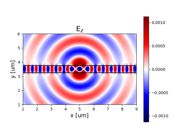
Real part of the z component of the electric field of the simulated simple waveguide.