2. Solving for modes of 2D Waveguides¶

A key component in many electromagnetic simulations (and in particular in photonics) is the waveguide. When simulating waveguiding structures, it is typically desirable to excite the structure by injecting a particular mode of a waveguide. In order to do so, we must first calculate that guided mode.

In this tutorial, you will learn how to calculate the modes and effective indices (of a 1D slice of) a 2D waveguide.

Note

Example Code

The code associated with this tutorial can be found in examples/waveguide_modes/wg_modes_2D.py

Note

Running the code

In order to run code written on top of EMopt, you are encouraged to take advantage of MPI for parallelism. EMopt is built on top of MPI from the ground up in order to accelerate its execution. In order to run this example using MPI on, for example, 4 cores, you would run the command:

$ mpirun -n 4 python wg_modes_2D.py

2.1. Setting up the Problem¶

The process of calculating waveguide modes is very similar to the process of running simulations. As in the case of setting up a simulation, in order to calculate a waveguide mode, we must first define the size and resolution of the system:

H = 6.0
dy = 0.02
wavelength = 1.55

Notice that we only specified a height and a single spatial step size. This is because the mode of a 2D structure is computed for a 1D slice.

2.2. Defining the Waveguide¶

We now need to define the material distribution of the waveguide for which modes will be calculated. To do this, we specify a 2D structure and then take a 1D slice from it. Because we are only taking a slice from it, the width along the x direction does not really matter.

To make things interesting, let us define a waveguide consisting of ridge-like refractive index profile:

w_wg_out = 2.0
w_wg_in = 0.4

# Define rectangles for the waveguide structure and cladding
wg_out = emopt.grid.Rectangle(0, H/2, 1.0, w_wg_out)
wg_out.layer = 2; wg_out.material_value = 2.5**2

wg_in = emopt.grid.Rectangle(0, H/2, 1.0, w_wg_in)
wg_in.layer = 1; wg_in.material_value = 3.45**2

bg = emopt.grid.Rectangle(0, H/2, 1.0, H)
bg.layer = 3; bg.material_value = 1.444**2

# Create a structured material which is just the ensemble of rectangles created above
# A slice from this StructuredMaterial will be used in the mode calculation
eps = emopt.grid.StructuredMaterial2D(1.0, H, dy, dy) # W and dx do not matter much
eps.add_primitive(wg_out); eps.add_primitive(wg_in); eps.add_primitive(bg)

mu = emopt.grid.ConstantMaterial2D(1.0)

This structure consists of three rectangles: first, a larger 2 μm tall lower-index rectangle is defined which consitutes a cladding for the waveguide. Next, a narrower 400 nm tall higher-index core is defined at the center of the simulation region. Finally an all-encompassing background refractive index is defined using a third rectangle.

In order to actually generate the material distribution that will be used in the mode solver, we created a emopt.grid.StructuredMaterial2D object to which we passed the previously instantiated rectangles. This defines the permittivity distribution. EMopt also expects a permeability distribution. As is frequently the case, we let the permeability be uniformly equal to 1.0. This is easily achieved using a emopt.grid.ConstantMaterial2D as depicted above.

At this point, we have a 2D structure. The mode solver only cares about 1D slices, however. We can specify which 1D slice to take by creating an appropriate emopt.misc.DomainCoordinates object:

mode_line = emopt.misc.DomainCoordinates(0.5, 0.5, 0, H, 0.0, 0.0, 1.0, dy, 1.0)

The emopt.misc.DomainCoordinates object can be used to define 1D, 2D, and 3D domains/regions. In this case, we define a 1D domain by specifying min and max coordinates for x and z which are the same (and hence have zero width). It is important to note that the spatial step size for x and z can be chosen to be anything other than zero in this case.

2.3. Defining and Running the Mode Solver¶

With the structure defined, all that remains is to setup and run the mode solver. This simply involves instantiating the desired mode solver and passing the appropriate arguments (wavelength, permittivity, permeability, domain of the slice, etc):

neigs = 8
modes = emopt.modes.ModeTE(wavelength, eps, mu, mode_line, n0=3.0, neigs=neigs)
modes.build() # build the eigenvalue problem internally
modes.solve() # solve for the effective indices and mode profiles

There are a few important things to note here. First, when calculating waveguide modes, we must specify how many modes to compute. Calculating mode modes can lead to modest increases in calculation time. Next, it is typically a good idea to specify a guess for the effective indices of the modes (given by the n0 argument). The mode solver will try to find modes with effective indices which are close to this value. Typically, the effective index of the modes will decrease with higher mode number. In general, it is a good idea to choose a value for n0 which is close to the highest refractive index in the simulation.

Finally, when calculating modes in 2D, we must specify whether we want to calculate transverse electric (TE) modes or transverse magnetic (TM) modes. In this case we chose TE, but we could have equally chosen TM by specifying emopt.modes.ModeTM instead (everything else would remain unchanged).

2.4. Visualizing the results¶

The results of the mode solver are made accessible through the emopt.modes.ModeTE.get_field_interp() function and the emopt.modes.ModeTE.neff variable. The former gives access to the calculating modal fields while the latter is an array containing the calculated effective indices. Note that neff is an array whose length matches the supplied number of eigenvalues, neigs.

There are two important characteristics which distinguish emopt.modes.ModeTE.get_field_interp() from its FDFD_TE counterpart. First, it is safe to get the modal fields from within a NOT_PARALLEL block (the results are saved for non-parallel interaction immediately after solving for them). Second, in addition to passing a desired field component, a mode index must be specified which specifies which mode’s fields are retrieved.

For this mode calculation, we will first print out the effective indices and then view the calculated mode profiles:

if(NOT_PARALLEL):
    import matplotlib.pyplot as plt

    # print out the effective indices
    print('          n_eff          ')
    print('-------------------------')
    for j in range(neigs):
        n = modes.neff[j]
        print('%d : %0.4f  +  %0.4f i' % (j, n.real, n.imag))

    # plot the refractive index and mode profiles
    f, axes = plt.subplots(3,1)
    for j in range(3):
        i = modes.find_mode_index(j)
        Ez = modes.get_field_interp(i, 'Ez')
        x = np.linspace(0, H, mode_line.Ny)
        eps_arr = eps.get_values_in(mode_line, squeeze=True)

        ax = axes[j]
        ax.plot(x, np.abs(Ez), linewidth=2)
        ax.set_ylabel('E$_z$ (TE$_%d$)' % j, fontsize=12)
        ax.set_xlim([x[0], x[-1]])

        ax2 = ax.twinx()
        ax2.plot(x, np.sqrt(eps_arr.real), 'r--', linewidth=1, alpha=0.5)
        ax2.set_ylabel('Refractive Index')

    axes[2].set_xlabel('x [um]', fontsize=12)
    plt.show()

Running this tutorial will generate and output the following effective index data to your terminal:

        n_eff
-------------------------
: 3.2140  +  0.0000 i
: 2.5845  +  -0.0000 i
: 2.3698  +  -0.0000 i
: 2.2936  +  -0.0000 i
: 1.9733  +  -0.0000 i
: 1.7689  +  0.0000 i
: 1.4048  +  0.0000 i
: 1.3919  +  -0.0000 i

Furthermore, the code will produce the following plot of the simulate mode profiles:

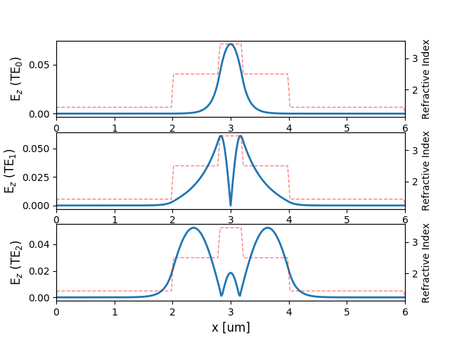
Electric field of the first three modes of a 2D waveguide overlayed with the waveguide’s refractive index profile.