3. Simulating a Waveguide in 2D Which is Excited With a Mode Source
In this tutorial, we will combined what we learned in the previous two tutorials in order to simulate a waveguide which is excited by a mode source. A mode source is a special type of current source distribution which unidirectionally injects the desired guided mode.
Note
Example Code
The code associated with this tutorial can be found in examples/simple_waveguide/simple_waveguide_mode.py
Note
Running the code
In order to run code written on top of EMopt, you are encouraged to take advantage of MPI for parallelism. EMopt is built on top of MPI from the ground up in order to accelerate its execution. In order to run this example using MPI on, for example, 4 cores, you would run the command:
$ mpirun -n 4 python simple_waveguide_mode.py
3.1. Setting up the Simulation Domain
As with the previous tutorials, our first step is to import the necessary
modules that we will use. In this example, those modules are emopt and
numpy:
import emopt
from emopt.misc import NOT_PARALLEL

import numpy as np
The NOT_PARALLEL variable that we import allows us to do non-parallel operations like plotting. We will return to this at the end of the tutorial!
After importing the necessary modules, we define the size and resolution of the simulation as well as the wavelength of the simulation source:
W = 5.0
H = 5.0
dx = 0.02
dy = 0.02
wlen = 1.55
In this tutorial, the simulation domain (including perfectly matched layers) will be 5 μm by 5 μm and the spatial grid step will be 20 nm. Based on our chosen wavelength of 1.55 μm, this simulation resolution yields 22 grid cells per wavelength in the high index material, which should ensure that the simulation is reasonably accurate.
With the simulation parameters chosen, we can instantiate our simulation object. In this tutorial, we will be performing a 2D transverse electric field simulation (i.e. the simulated field components are \(E_z\), \(H_x\), \(H_y\)):
sim = emopt.fdfd.FDFD_TE(W, H, dx, dy, wlen)

W = sim.W
H = sim.H
M = sim.M
N = sim.N
Typically, an integer number of grid cells of the chosen dimension will not fit in the simulation domain. EMopt will “stretch” the simulation domain such that it does contain an integer number of grid cells. This results in an updated simulation width and height which we retrieve from the sim object. Similarly, we retrieve the number of grid cells along x (N) and along y (M) from the sim object.
With the simulation object instantiated, we are ready to start defining simulation geometry!
3.2. Defining Materials and Structures
In order to simulate a waveguide, we need to define the waveguide size and material value. The waveguide in this tutorial is a 220 nm wide silicon waveguide (index ~3.45). The waveguide is clad on top and bottom by silicon dioxide (index ~1.44). In order to define this material distribution, we create a rectangle for the waveguide and a second rectangle which spans the whole simulation domain. These are combined to form a permittivity distribution:
# Material constants
n0 = 1.44
n1 = 3.45

# set a background permittivity of 1
eps_background = emopt.grid.Rectangle(W/2, H/2, 2*W, H)
eps_background.layer = 2
eps_background.material_value = n0**2

# Create a high index waveguide through the center of the simulation
h_wg = 0.22
waveguide = emopt.grid.Rectangle(W/2, H/2, W*2, h_wg)
waveguide.layer = 1
waveguide.material_value = n1**2

# Create the a structured material which holds the waveguide and background
eps = emopt.grid.StructuredMaterial2D(W, H, dx, dy)
eps.add_primitive(waveguide)
eps.add_primitive(eps_background)
Similarly, we need to define a permeability distribution. This can be done in
an identical manner. In this tutorial, we want the permeability to be uniformly
1. This is easily accomplished by creating a
emopt.grid.ConstantMaterial2D object:
mu = emopt.grid.ConstantMaterial2D(1.0)
With the permittivity and permeability distribution formed, we can pass them onto the solver, thus completing the process of defining the simulation geometry:
sim.set_materials(eps, mu)
Now we just need to set up the sources which will excite the waveguide we have just defined!
Note
For more complicated geometries, emopt.grid.Rectangle may be
insufficient. In such cases, the emopt.grid.Polygon class provides
increased flexibility.
3.3. Defining the Simulation Mode Source
Our goal in this tutorial is to excite the fundamental mode of the waveguide. In order to do this, we have to first calculate the mode of the waveguide that we want to excite. We can then use calculate the current density distribution which will excite that waveguide mode.
In order to calculate the waveguide mode, we take a vertical slice of the simulation and pass it to EMopt’s mode solver:
src_line = emopt.misc.DomainCoordinates(W/4, W/4, sim.w_pml[2], H-sim.w_pml[3],
                                        0.0, 0.0, dx, dy, 1.0)

# setup, build the system, and solve
mode = emopt.modes.ModeTE(wlen, eps, mu, src_line, n0=n1, neigs=4)
mode.build()
mode.solve()
For the purpose of solving for the waveguide mode, the x position of the slice
does not matter. However, we will use the same DomainCoordinates to
specify where in the simulation the source plane will be placed, thus in this
case the x position does matter. For this tutorial, the source plane will span
the y dimension of the simulation (excluding the perfectly matched layers which
are automatically defined) and will be positioned at \(x=W/4\).
With the waveguide mode calculated, all we need to do is passed the built and solve mode solver to our simulation object. The simulation object will take care of generating the necessary current distribution arrays:
# after solving, we cannot be sure which of the generated modes is the one we
# want.  We find the desired TE_X mode
mindex = mode.find_mode_index(0)

# set the sources using our mode solver
sim.set_sources(mode, src_line, mindex)
Note that when setting the sources using a mode solver, we must also provide
the DomainCoordinates which specifies the location of the mode source
as well as the index of the mode we want to excite. For the fundamental mode,
this index is typically 0, however to be safe, in this tutorial we use the
mode.finde_mode_index() function to get the \(TE_0\) mode.
3.4. Running the Simulation
With the simulation geometry and sources defined, we are read to run the simulation and visualize the results. In order to run a simulation, we first build the problem and then solve for the fields:
sim.build()
sim.solve_forward()
Depending on how powerful your computer is and how many processes you run it with, these two function calls should only take ~10 seconds.
Once the solve_forward() function is complete, we can retrieve the
simulated fields in a desired area of the simulation domain by specifying the
region using emopt.misc.DomainCoordinates and then calling the
emopt.fdfd.FDFD_TE.get_field_interp() function. In our case, we want to
retrieve the \(E_z\) component of the field:
sim_area = emopt.misc.DomainCoordinates(1.0, W-1.0, 1.0, H-1.0, 0.0, 0.0, dx, dy, 1.0)
Ez = sim.get_field_interp('Ez', sim_area)
The variable Ez will be a numpy array with dimensions which match sim_area. With the field retrieved, we are free to do with it as we wish. In this case, let us visualize them using matplotlib:
if(NOT_PARALLEL):
    import matplotlib.pyplot as plt

    extent = sim_area.get_bounding_box()[0:4]

    f = plt.figure()
    ax = f.add_subplot(111)
    im = ax.imshow(Ez.real, extent=extent,
                            vmin=-np.max(Ez.real)/1.0,
                            vmax=np.max(Ez.real)/1.0,
                            cmap='seismic')
    f.colorbar(im)
    ax.set_title('E$_z$', fontsize=18)
    ax.set_xlabel('x [um]', fontsize=14)
    ax.set_ylabel('y [um]', fontsize=14)
    plt.show()
When doing plotting like this, it is important to run all of the plotting code
in an if(NOT_PARALLEL) block. This is because some simulation results
may only be stored in the rank 0 process and also because we typically don’t
want to plot things N times. NOT_PARALLEL ensures that the plot is
generated only once.
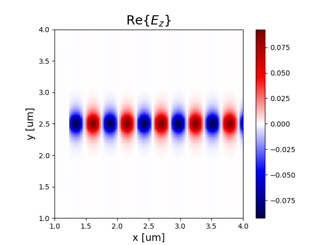
Real part of the electric field of a waveguide which is excited by a mode source.