4. Optimizing a Grating Coupler

In previous tutorials, we learned how to setup and run simulations. These simulations form the backbone of electromagnetic optimizations and typically account for a large part of setting up and running an optimization.

In this tutorial, we will demonstrate in detail how what we learned in the previous tutorials can be used to optimize a grating coupler in two dimensions. This structure consists of a waveguide with (initially periodic) which is situated above a thicker silicon slab and which is clad in silicon dioxide.

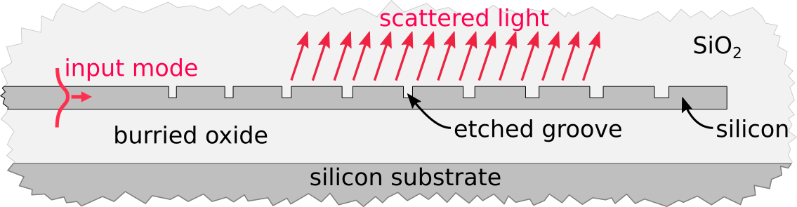
Diagram of a typical partially etched grating coupler.

The goal of the optimization will be to modify the grating design in order to maximize the coupling efficiency of the grating into a desired output Gaussian beam. The parameters of the grating that we will modify are the widths and local periodicity of the etched grooves, the depth of the etch, and the thickness of the burried oxide.

In order to optimized electromagnetic devices, EMopt calculates gradients using the adjoint method [1]. These gradients can be used in conjunction with off-the-shelf minimization algorithms for optimization. Broadly speaking, the process of optimizing a device like this grating coupler can be broken into 4 parts:

1. Define the structure to be optimized and set up a simulation of that strucutre.
2. Define the design parameters and specify how those design parameters modify the structure
3. Define a figure of merit which describes the performance of the device and its derivative with respect to the electric and magnetic fields.
4. Verify that the gradients of the figure of merit are accurate.
5. Run the optimization using a minimization algorithm of your choice.

In this tutorial, we will work through each of these steps in detail. By the end, you should have a good understanding of how EMopt can be used to rapidly optimized electromagnetic structures with many degrees of freedom.

Note

Example Code

The code associated with this tutorial can be found in examples/Silicon_Grating_Coupler/gc_opt.py

Note

Running the code

In order to run code written on top of EMopt, you are encouraged to take advantage of MPI for parallelism. EMopt is built on top of MPI from the ground up in order to accelerate its execution. In order to run this example using MPI on, for example, 14 cores, you would run the command:

$ mpirun -n 14 python gc_opt.py

Note that the simulations performed as a part of this optimization are quite a bit larger than those in the previous tutorials. Running the code with more processes and on a fast machine is recommended.

Warning

Previous Tutorials

This tutorial assumes you have completed the previous tutorials on 2D simulation with EMopt. It is highly recommended you work through these tutorials first.

4.1. Imports and File Stucture

In this tutorial, we will be relying primarily on EMopt modules and numpy:

import emopt
from emopt.misc import NOT_PARALLEL
from emopt.adjoint_method import AdjointMethodPNF

# We define the desired Gaussian modes in a separate file
from mode_data import Ez_Gauss, Hx_Gauss, Hy_Gauss

import numpy as np
from math import pi

Notice a few new things here. First, we have imported a class called AdjointMethodPNF. This is an interface that we will soon override in order to define import details of the optimization. Second, we import a set of functions Ez_Gauss(), etc. These functions can be found in the example folder and simply generate a Gaussian field profile that we will use in our figure of merit calculation (more on this soon).

Beyond this single external set of functions, the entire optimization will be setup and run from a single python script (gc_opt.py). The structure of this files is as follows:

class SiliconGratingAM(AdjointMethodPNF):
    ## Define the details of the adjoint method for our grating coupler
    def __init__(self, ...):
        ## Initialize variables
        # [PART 5]

        ## Setup FOM fields
        # [PART 8]

    def update_system(self, params):
        ## given design parameter values, update the system
        # [PART 6]
        pass

    def calc_f(self, sim, params):
        ## calculate the value of the figure of merit
        # [PART 9]
        pass

    def calc_dfdx(self, sim, params):
        ## calculate the derivatives of the figure of merit with respect to
        ## the electric and magnetic fields (df/dEz, df/dHx, and df/dHy)
        # [PART 10]
        pass

    def calc_grad_y(self, sim, params):
        ## calculate the derivative of the figure of merit with respect to
        ## the design parameters
        # We won't use this in this tutorial
        pass

    def get_update_boxes(self, sim, params):
        ## define what regions of the simulation domain are affected by
        ## changes to the design variables
        # [PART 7]
        pass

def plot_update(params, fom_list, sim, am):
    ## Plot the structure, fields, and figure of merit after each iteration
    # [PART 13]
    pass

if __name__ == "__main__":
    ## Setup the simulation domain
    # [PART 1]

    ## Setup the geometry
    # [PART 2]

    ## Setup the sources
    # [PART 3]

    ## Setup saved fields
    # [PART 4]

    ## Instantiate the AdjointMethod and verify gradient accuracy
    # [PART 11]

    ## Run the optimization
    # [PART 12]

This file structure is fairly standard for optimizations based on EMopt. In the next sections of this tutorial, we will fill in each part of this file (denoted by [PART #]) and discuss some of the finer details.

4.2. Setting up the Simulation

4.2.1. Creating the Simulation Domain

Our first step is to setup the simulation domain and define the grating coupler structure. For 1550 nm light, grating couplers are typically ~20 μm long. In order to full encompass this length and allow the grating to grow a bit, we will make the simulation domain 26 μm long. Similarly, in order to allow enough room for the burried oxide which is typically ~2 μm thick and also allow the beam to propagate a few micron, we will make the simulation domain 8 um tall. In order to ensure that the simulation is reasonably accurate, we choose a grid spacing of 20 nm along x and y. Putting all this together, we can instantiate our simulation object by writing the following code in PART 1 of our optimization script:

wavelength = 1.55
W = 28.0
H = 8.0
dx = 0.02
dy = dx

# create the simulation object.
# TE => Ez, Hx, Hy
sim = emopt.fdfd.FDFD_TE(W, H, dx, dy, wavelength)

# Get the actual width and height
W = sim.W
H = sim.H
M = sim.M
N = sim.N
w_pml = sim.w_pml[0] # PML width which is the same on all boundaries by default

In the last line, we retrieve the size of the perfectly matched layers which by default is the same on all boundaries. This PML width will come in handy in a bit when we define the source and figure of merit plane.

4.2.2. Defining the Simulation Structure

With the simulation domain setup, we can now begin to specify the geometry of the system. Our first step is to specify the material values for the system:

n_si = emopt.misc.n_silicon(wavelength)
eps_core = n_si**2
eps_clad = 1.444**2

# the effective indices are precomputed for simplicity.  We can compute
# these values using emopt.modes
neff = 2.86
neff_etched = 2.10
n0 = np.sqrt(eps_clad)

Here, we make use of the n_silicon() function to get the value of the refractive index of silicon at 1550 nm. Furthermore, we hardcode two addition refractive indices (neff and neff_etched) which are precomputed values for the effective index of the unetched and etched sections of the grating coupler. For the purpose of this tutorial, we precompute these values. In many cases, it may be more desirable to directly calculate them using modes.

Our next step is to define the grating coupler structure. As depicted above, the grating coupler consists of a waveguide with etched grooves. To define this structure, we will create a rectangle of silicon which defines the input waveguide and unetched portion of the grating and then a list of smaller rectangles of silicon dioxide which define the etched slots of the grating. The initial periodicity of these slots will be calculated uing the effective indices and desired angle (which in this case is 8 degrees in oxide). Our first step is to define the waveguide parameters and calculate the grating period in PART 2 of our script:

# set up the initial dimensions of the waveguide structure that we are exciting
h_wg = 0.28
h_etch = 0.19 # etch depth
w_wg_input = 5.0
Ng = 26 #number of grating teeth

# set the center position of the top silicon and the etches
y_ts = H/2.0
y_etch = y_ts + h_wg/2.0 - h_etch/2.0

# define the starting parameters of the partially-etched grating
# notably the period and shift between top and bottom layers
df = 0.8
theta = 8.0/180.0*pi
period = wavelength / (df * neff + (1-df)*neff_etched - n0*np.sin(theta))

Next, we build up the grating slots. There will be a total of Ng grating slots, each of with is a rectangle with the desired initial width (corresponding to a duty factor of 80%) and permittivity:

# We now build up the grating using a bunch of rectangles
grating_etch = []

for i in range(Ng):
    rect_etch = emopt.grid.Rectangle(w_wg_input+i*period, y_etch,
                                     (1-df)*period, h_etch)
    rect_etch.layer = 1
    rect_etch.material_value = eps_clad
    grating_etch.append(rect_etch)

In general, when optimizing grating couplers an initial duty factor >~60% should be used to ensure that unwanted local minima are avoided. Notice that the layer of the grating slots is set to 1. This will be the lowest layer value in our stack to ensure that the grating slot rectangles are on top of the waveguide.

With the grating slots defined, we can finish off the grating by creating the background waveguide that is etched:

# grating waveguide
Lwg = Ng*period + w_wg_input
wg = emopt.grid.Rectangle(Lwg/2.0, y_ts, Lwg, h_wg)
wg.layer = 2
wg.material_value = eps_core

In terms of the structure, all that remains is the substrate and cladding. Both are defined using rectangles of the appropriate size and position. In this optimization, we will begin with a burried oxide thickness (distance between the bottom of the grating and silicon substrate) of 2 μm. The top and bottom cladding, meanwhile, will be oxide:

# define substrate
h_BOX = 2.0
h_subs = H/2.0 - h_wg/2.0 - h_BOX
substrate = emopt.grid.Rectangle(W/2.0, h_subs/2.0, W, h_subs)
substrate.layer = 2
substrate.material_value = eps_si # silicon

# set the background material using a rectangle equal in size to the system
background = emopt.grid.Rectangle(W/2,H/2,W,H)
background.layer = 3
background.material_value = eps_clad

With the different components of the structure defined, all that remains is to combine them together into a permittivity distribution. We do this using a StructuredMaterial2D:

eps = emopt.grid.StructuredMaterial2D(W,H,dx,dy)

for g in grating_etch:
    eps.add_primitive(g)

eps.add_primitive(wg)
eps.add_primitive(substrate)
eps.add_primitive(background)

Getting the values of this StructuredMaterial2D yields the following permittivity distribution:

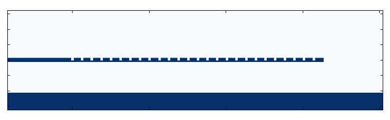
Initial permittivity distribution of the grating coupler.

You may notice that we chose the simulation width such that there is a decent amount of space after the end of the grating. This ensures that there is enough space for grating to grow during the optimization.

In addition to the permittivity distribution, we need to define a permeability distribution. In this example, the permeability is uniformly equal to one:

mu = emopt.grid.ConstantMaterial2D(1.0)

With both permittivity and permeability defined, we complete the generation of the structure by passing eps and mu to the simulation object.

sim.set_materials(eps, mu)

This completes PART 2 of our script.

4.2.3. Setting the Simulation Sources

Our next step is to specify the simulation sources. When simulating single polarization grating couplers using a 2D approximation, we typically have two options as to how we inject power into the structure. We can either inject the fundamental TE mode of the input waveguide and measure the field scattered into free-space modes or we can inject the desired field (a Gaussian beam) and measure the field coupled into the grating coupler waveguide.

In this optimization, we will be using the former method (injecting power into the grating coupler waveguide). In order to do this, we will solve for the modes of the input waveguide to the grating coupler and then extract the corresponding current density distributions which will surve as the source to our simulations.

The process for doing this is the same in the previous tutorial. First, we create a DomainCoordinates which defines the vertical slice of the simulation where light will be injected in PART 3 of our script:

w_src= 3.5

# place the source in the simulation domain
src_line = emopt.misc.DomainCoordinates(w_pml+2*dx, w_pml+2*dx, H/2-w_src/2,
                                        H/2+w_src/2, 0, 0, dx, dy, 1.0)

Next, We setup the mode solver object by passing the permittivity, permeability, and source line objects. Note that we are simulating TE fields so we need to use a TE source:

# Setup the mode solver.
mode = emopt.modes.ModeTE(wavelength, eps, mu, src_line, n0=n_si, neigs=4)

In addition, we also specify a guess for the effective index of the mode we are looking for. Typically, you should set this to be equal to or greater than the desired effective index. Since we don’t typically know this value before running the mode solver, using the refractive index of the highest index material is a safe choice.

Finally, in order to use the mode solver, we build and solve for the mode and then pass it to our simulation object to set the sources:

mode.build()
mode.solve()

# at this point we have found the modes but we dont know which mode is the
# one we fundamental mode.  We have a way to determine this, however
mindex = mode.find_mode_index(0)

# set the current sources using the mode solver object
sim.set_sources(mode, src_line, mindex)

Here, modes.ModeTE.build() generates the generalized eigenvalue problem which is solved and then modes.ModeTE.solve() actually solves for the modes and effective indices (eigenfunctions and eigenvalues). The mode solver solves for multiple modes and stores them internally in an array. In order to get the fundamental mode, we use the mode.ModeTE.find_mode_index() function to figure out which index of that array contains the fundamental mode (i.e. mode 0).

4.2.4. Specifying Fields to Save (i.e., Field Monitors)

The last step in setting up the underlying simulation for our optimization is to define where in the simulation domain we want to record the fields. To do this, we simply define DomainCoordinates objects and pass them to the simulation object. In this optimization, we want to record the fields in a 1D slice which will be used to calculate the coupling efficiency of the grating coupler and a second 2D domain which records the fields in the simulation for the purpose of visualization. We create these DomainCoordinates objects in PART 4 of our script:

mm_line = emopt.misc.DomainCoordinates(w_pml, W-w_pml, H/2.0+2.0, H/2.0+2.0, 0, 0,
                                       dx, dy, 1.0)
full_field = emopt.misc.DomainCoordinates(w_pml, W-w_pml, w_pml, H-w_pml, 0.0, 0.0,
                                          dx, dy, 1.0)

Finally, we assign these DomainCoordinates objects to the field_domains property of our simulation object:

sim.field_domains = [mm_line, full_field]

Now, whenever we run a simulation of our grating coupler, the FDFD solver will automatically save the fields in these two domains. These fields can be accessed using the saved_fields property of the simulation object.

Note

Technically, using the field_domains and save_fields properties are unnecessary. Alternatively, we could just use the fdfd.FDFD_TE.get_field_interp() function whenever we want to work with the fields. The disadvantage this function, however, is that it must be called on all processors. This is because the fields are distributed across multiple MPI processes. When using the field_domains property, however, the solver will automatically call fdfd.FDFD_TE.get_field_interp() immediately after the simulation has finished and save those results on the rank 0 process. These fields can then be retrieved at any time, even in a non-parallelized block of code. This allows us to largely avoid the complexity of working with parallelized code.

4.2.5. Finalizing the Simulation Setup

At this point, we are finished setting up our grating coupler simulation. We can now build the system in preparation for running simulations also in PART 4 of our script:

sim.build()

In principle, we could now run a simulation of the structure using the fdfd.FDFD_TE.solve_forward() function and visualize the results. Doing so yields the following field:

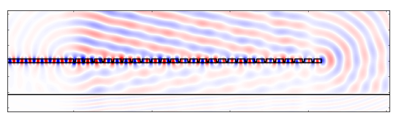
Plot of \(E_z\) of the initial grating coupler structure.

And there you go! We have a simulated grating coupler.

4.3. Setting up the optimization: Defining an AdjointMethod

The simulation that we just set up forms the foundation of our optimization. At a high level, the optimization is just (intelligently) tweaking the the structure in order to “improve” the fields that come out of the simulation. In many cases, setting up the simulation is the most labor intensive part of putting together an optimization!

In this section, we will walk through how to construct the second major component of our grating coupler optimization: the gradient calculation. In order to rapidly optimize electromagnetic structures EMopt uses a gradient-based approach. In fact, the core purpose of EMopt is to calculate derivatives of figures of merits for electromagnetic devices.

The basic idea (discussed in detail in [1] and [2]) is that we specify a function of the electric fields, magnetic fields, and design parameters \(F(\mathbf{E}, \mathbf{H}, \vec{p})\) which is a measure of the performance of our device. We then take the gradient of this function with respect to the design parameters,

\[\nabla_\vec{p} F = \left[\frac{\partial F}{\partial p_1}, \frac{\partial F}{\partial p_2}, \frac{\partial F}{\partial p_3}, \dots\right]\]

This gradient effectively tells us which direction in the design space to search for the optimal device. We can use this gradient in conjunction with efficient minimization algorithms like BFGS (provided by scipy.optimize) in order to find the set of design variables \(\vec{p}\) which yield an efficient structure.

It turns out that calculating the gradient \(\nabla_\vec{p} F\) is a bit tricky. This is largely a result of (1) the fact that simulations of Maxwell’s equations are quite costly and (2) it is difficult to displace boundaries of a structure in a smooth way, especially when using finite-difference methods for the underlying simulations. This is where EMopt shines. EMopt provides us with an implementation of the adjoint method which allows us to calculate the gradient of our figure of merit using only two simulations. Furthermore, EMopt implements boundary smoothing techniques (discussed in ref [2]) which ensures that changes to the boundaries of whatever structure we simulate are differentiable.

The latter functionality has already been taken care of for us when we chose to use the StructuredMaterial2D class for defining the permittivity distribution. This class applies boundary smoothing to the constituent shapes when generating the material distribution. As for the provess of using EMopt’s adjoint method implementation, we need to do a bit more work. In particular, we need to define our own AdjointMethod class.

4.3.1. Overview of the AdjointMethod Class

In order to optimize our electromagnetic device, we need to specify three important things:

1. Parameterization: Define a set of design parameters (numbers) which

   affect the shape of the device in some way.

2. Figure of Merit: The function that describes the performance of the

   device that we will minimize by changing the design parameters.

3. Analytic Derivative of the Figure of Merit: The derivative of the

   figure of merit with respect to the electric and magnetic fields. This is needed by the adjoing method in order to calculate the derivative of the FOM with respect to the design parameters.

Once we have taked care of these three things, we can efficiently calculate the gradients of our figure of merit. In order to do these things, we create a custom implementation of an AdjointMethod class. EMopt defines a couple different base classes which take care of most of the heavy lifting; we just need to override a few key methods.

Let us go ahead and define this new class and its constructor (PART 5 and 8 of our script):

class SiliconGratingAM(AdjointMethodPNF):

    def __init__(self, sim, grating_etch, wg, substrate, y_ts, w_in, h_wg, H, Ng,
                 eps_clad, mm_line):
        # Call super class constructor--important!
        super(SiliconGratingAM, self).__init__(sim, step=1e-10)

        # save the variables for later
        self.grating_etch = grating_etch
        self.y_ts = y_ts
        self.w_in = w_in
        self.h_wg = h_wg
        self.H = H
        self.Ng = Ng
        self.wg = wg
        self.substrate = substrate

        self.mm_line = mm_line
        self.current_fom = 0.0

        # desired Gaussian beam properties used in mode match
        theta = 8.0/180.0*pi
        match_w0 = 10.4/2.0
        match_center = 11.0

        # Define the desired field profiles
        # We use a tilted Gaussian beam which approximates a fiber mode
        Ezm, Hxm, Hym = emopt.misc.gaussian_fields(mm_line.x-match_center,
                                                      0.0, 0.0, match_w0,
                                                      theta, sim.wavelength,
                                                      np.sqrt(eps_clad))

Here, we extend a class defined by EMopt called AdjointMethodPNF. “PNF” stands for “power normalized function” and is used for figures of merit which consist of functions which are normalized with respect to the source power of the simulation. In this optimization, our figure of merit will be the coupling efficiency into a desired output mode; in order to calculate an efficiency we will need this power normalization. EMopt contains a number of other adjoint method classes. See the modules documentation for adjoint_method for details.

The constructor we have just defined serves two primary functions: (1) it stores important variables relating to the grating coupler structure that we will need when defining the parameterization, figure of merit, etc and (2) it generates the reference electric and magnetic fields that we will use in the calculation of our figure of merit.

Next, we will learn how to define the parameterization, figure of merit, and analytic derivatives needed to complete our AdjointMethodPNF implementation. We do this by overriding a couple of functions.

4.3.2. Defining the Parameterization

The goal of our grating coupler optimization is to apodize the grating and choose the optimal etch depth and BOX thickness. As such, the design parameters of our system will be related to the widths and periodicity of the etched slots, the etch depth, the BOX thickness, and a horizontal shift of the whole grating:

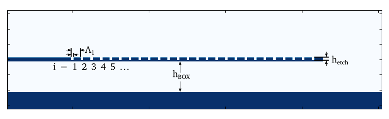
Diagram of grating parameterization.

Specifically, for our parameterization we will assign an integer index to each tooth in the grating. The local “period” and gap width along the grating will be defined as a Fourier series function of this index:

\[\Lambda(i) = \sum\limits_{i=1}^{N_F} \left[a_i \sin(\frac{\pi}{N_g}i) + b_i \sin(\frac{\pi}{N_g}i)\right]\]

\[w_\mathrm{g}(i) = \sum\limits_{i=1}^{N_F} \left[c_i \sin(\frac{\pi}{N_g}i) + d_i \sin(\frac{\pi}{N_g}i)\right]\]

Here, \(i\) is the grating index and \(N_g\) is the total number of periods in the grating. The Fouriet coefficients \(a_i\), \(b_i\), \(c_i\), and \(d_i\) are design parameters of our optimization. By manipulating them, we will modify how the etched slots evolve along the length of the grating.

You may wonder why we don’t simply set the individual slot widths and spacings as the design parameters. In some cases we will do this (for example when we want to specify feature size constraints, this is an appropriate parameterization). In this case, however, we choose a Fourier parameterization with a limited number of terms as it forces the grating to take on a gradually changing shape. This gradual change is important since (as we will discuss in just a moment) we are trying to match to a smoothly varying Gaussian beam. Abrupt changes to the grating structure will not lead to a field that matches well to a Gaussian beam, and so we choose a parameterization which prevents that from happening. This has the added benefit that it typically leads to optimization problems with fewer parameters which exhibit faster convergence (fewer interations).

In order to actually define the parameterization in code, we need to implement the adjoint_method.AdjointMethod.update_system() function. This function takes a single 1D array containing the current values of the design parameters as an argument and updates the simulation structure accordingly. We begin by extracting the different types of design parameters from the input array (in PART 6 of our script):

def update_system(self, params):
    coeffs = params
    Nc = self.Nc

    h_etch = params[-3]
    h_BOX = params[-1]
    x0 = self.w_in + params[-2]

Next we need to update the etched slots. We do this in two steps: first, we define a little function that computes the desired Fourier series. Next, we loop through the grating etch rectangles and resize and reposition them based on this Fourier series:

fseries = lambda i, coeffs : \
          coeffs[0] + np.sum([coeffs[j] *np.sin(pi/2*i*j*1.0/self.Ng) \
                              for j in range(1,Nc)]) \
                    + np.sum([coeffs[Nc + j] * np.cos(pi/2*i*j*1.0/self.Ng) \
                              for j in range(0,Nc)])
for i in range(self.Ng):
    w_etch = fseries(i, coeffs[0:2*Nc])
    period = fseries(i, coeffs[2*Nc:4*Nc])

    # update the rectangles
    self.grating_etch[i].width  = w_etch
    self.grating_etch[i].height = h_etch
    self.grating_etch[i].x0     = x0 + w_etch/2.0
    self.grating_etch[i].y0     = self.y_ts + self.h_wg/2.0 - h_etch/2.0

    x0 += period

Finally, we need to update the BOX thickness as well as the length of the waveguide which is etched to form the grating:

# update the BOX/Substrate
h_subs = self.H/2.0 - self.h_wg/2.0 - h_BOX
self.substrate.height = h_subs
self.substrate.y0 = h_subs/2.0

# update the width of the unetched grating
w_in = x0
self.wg.width = w_in
self.wg.x0 = w_in/2.0

This takes care of the update_system() function. This is one of the most important functions we implement when setting up a simulation. It forms the connection between the design parameters and the actual simulated structure. It

Note

The update_system() function is called very frequently during the course of an optimization. As such, you should implement the update_system() function in a reasonably efficient way to minimize runtime. Typically this won’t actually require any additional consideration on your part.

In addition to update_system(), there is one additional function that we will implement related to the parameterization: the get_update_boxes() function. This function defines a box which defines what region in the simulation domain is modified by the design parameters. This function exists to speed up the gradient calculation. In order to handle completely arbitrary device parameterizations with minimal effort on the user’s part, EMopt calculates shape gradients using finite differences. This involves calculating material distributions, perturbing the design variables, and recalculating the material distributions. In order to speed up this calculation, we can restrict the recalculations to only the relevant part of the simulation domain.

In this case, changes to the Fourier coefficients, the etch depth, and grating shift will only affect the permittivity in the grating coupler itself. As such, for these design parameters we specify a box which encompasses the grating. For the BOX thickness, we use a box which encompasses the whol simulation for simplicity.

In terms of implementation, get_update_boxes() expects us to return a list of lists/tuples which contain 4 floating point values. These 4-float lists define the bounding boxes. In total, there need to be as many bounding boxes as there are design parameters. The positions of the bounding boxes in this list should match the positions of the design parameters in the params list.

For our optimization, we do this in PART 7 of our script:

def get_update_boxes(self, sim, params):
    h_wg = self.h_wg
    y_wg = self.y_ts
    lenp = len(params)

    # define boxes surrounding grating
    boxes = [(0, sim.W, y_wg-h_wg, y_wg+h_wg) for i in range(lenp-1)]

    # for BOX, update everything (easier)
    boxes.append((0, sim.W, 0, sim.H))
    return boxes

This completes our parameterization-related tasks.

4.3.3. Defining the Figure of Merit

Our next step is to define the figure of merit. The purpose of our grating coupler is to couple 1550 nm light into a single mode optical fiber (SMF-28). A good approximation for the mode of an SMF-28 fiber is a Gaussian beam with a full width at half maximum (FWHM) of 10.4 μm. In order to maximize the coupling of light scattered by our grating coupler into this mode, our figure of merit will be the mode match between the generated fields and this Gaussian beam. Assuming no fields are reflected back towards the grating, the mode match equation is given by

\[\eta(\mathbf{E}, \mathbf{H}) = \frac{1}{4}\frac{\left|\int dx \mathbf{E}\times\mathbf{H}_m\right|^2}{P_\mathrm{src} P_m}\]

where \(\mathbf{E}\) is the simulated electric field, \(\mathbf{H}_m\) is the reference (desired) magnetic field, \(P_\mathrm{src}\) is the total source power (power in the injected waveguide mode), and \(P_m\) is the power residing in the reference fields. When the reference fields consist of a single wavevector (i.e. they are a single mode of the system), this function yields the fraction of power in the simulated fields which is contained in the desired field. When the reference field is not described by a single wavevector, this function is a slightly more approximate description of coupling efficiency. For our approximate fiber mode, this function will do a good job of representing the coupling efficiency.

We can implement this figure of merit in our code in two steps. The first step, which we have actually already completed, is to define the reference fields. This is accomplished at the end of our AdjointMethod constructor (PART 8) with the following code:

Ezm, Hxm, Hym = emopt.misc.gaussian_mode(mm_line.x-match_center,
                                         0.0, match_w0,
                                         theta, sim.wavelength,
                                         np.sqrt(eps_clad))
self.mode_match = emopt.fomutils.ModeMatch([0,1,0], sim.dx, Ezm=Ezm, Hxm=Hxm, Hym=Hym)

Here we generate the refernce fields with the help of the misc.gaussian_mode() function. These fields are then used to instantiate a ModeMatch object as shown above. The ModeMatch class is one of the most essential classes when it comes to defining figures of merit in silicon photonics. It facilitates not only the calculation of mode matches, but also the calculation of its derivative with respect to the electric and magnetic fields.

In order to actually set the figure of merit for our AdjointMethodPNF, we simply override the function calc_f(). This function has two arguments, the simulation object and the current array of design parameters, and returns the current value of the figure of merit without any power normalization. In other words, if the figure of merit is given by

\[F(\mathbf{E}, \mathbf{H}) = \frac{f(\mathbf{E}, \mathbf{H})}{P_\mathrm{src}}\]

then this function calculates \(f(\mathbf{E}, \mathbf{H})\). Whenever we wish to calculate the figure of merit in the future, we will use the adjoint_method.AdjointMethod.fom() function which internally calls our calc_f() function and normalizes it with respect to the source power.

In this case, we want to return the (non-normalized) mode match between the simulated fields and the desired Gaussian fields. The calc_f() function (PART 9) which accomplish this is relatively simple:

def calc_f(self, sim, params):
    # Get the fields which were recorded
    Ez, Hx, Hy = sim.saved_fields[0]

    # compute the mode match efficiency
    self.mode_match.compute(Ez=Ez, Hx=Hx, Hy=Hy)

    # we want to maximize the efficiency, so we minimize the negative of the efficiency
    self.current_fom = -self.mode_match.get_mode_match_forward(1.0)
    return self.current_fom

Here, the ModeMatch class is doing the bulk of the heavy lifting. You will notice that we made the mode match negative. The reason for this is that the optimizer will try to minimize our figure of merit. In order to maximize the mode match, we minimize the negative of the mode match.

This finished the process of defining our figure of merit. To recap: in order to define the figure of merit, we override the appropriate function of the AdjointMethod class. In this case, since our adjoint method implementation is based on the AdjointMethodPNF class, we implement the calc_f() function which simply retrieves the simulated fields and uses them to calculate the figure of merit (without power normalization).

4.3.4. Calculation the Derivative of the Figure of Merit

In order to complete our adjoint method implementation, we must supply the derivative of our figure of merit with respect to the electric and magnetic fields. Because we are working with TE fields, this means that we need to calculate the gradients \(\partial F/\partial \vec{E}_z\), \(\partial F/\partial \vec{H}_x\), and \(\partial F/\partial \vec{E}_y\).

Because we are using the ModeMatch class, this process is relatively straightforward. All we need to do is to override the calc_dfdx() function and generate 2D arrays which span the whole simulation domain. These arrays will contain the analytically calculated derivatives of the figure of merit with respect to E and H. We accomplish this in PART 10 with:

def calc_dfdx(self, sim, params):
    dFdEz = np.zeros([sim.M, sim.N], dtype=np.complex128)
    dFdHx = np.zeros([sim.M, sim.N], dtype=np.complex128)
    dFdHy = np.zeros([sim.M, sim.N], dtype=np.complex128)

    # Get the fields which were recorded
    Ez, Hx, Hy = sim.saved_fields[0]

    self.mode_match.compute(Ez=Ez, Hx=Hx, Hy=Hy)

    dFdEz[self.mm_line.j, self.mm_line.k] = -self.mode_match.get_dFdEz()
    dFdHx[self.mm_line.j, self.mm_line.k] = -self.mode_match.get_dFdHx()
    dFdHy[self.mm_line.j, self.mm_line.k] = -self.mode_match.get_dFdHy()

    return (dFdEz, dFdHx, dFdHy)

Note

Why are the derivatives 2D arrays which span the whole simulation?

These derivatives are taken with respect to the field values. Since we are working in a discretized space, this is equivalent to taking the derivative with respect to the field at each point in the grid.

How are these derivatives used?

The basic idea behind the adjoint method is that we run two simulations of the structure, and based on these two simulations we can calculate the full gradient of our figure of merit with respect to all of the design variables. One of these simulations, which we call the forward simulation, is simply a simulation of Maxwell’s equations. The second simulation, which we call the adjoint simulation, is a simulation of the transpose of Maxwell’s equations. It turns out (as a result of some basic math) that the current sources for this adjoint equation are exactly equal to the derivative of our figure of merit with respect to the field at each point in the grid.

In cases where you implement a different figure of merit, you will need to manually calculate the derivatives of your figure of merit with respect to the fields at each point in the grid. For example, let us consider the case where our figure of merit is given by:

\[F(\mathbf{E}) = \left|E_z\right|^2\]

In this case, the derivatives of our figure of merit are given by

\[\frac{\partial F}{\partial E_z}\bigg|_{i j} = \frac{\partial}{\partial E_z}\left(\left|E_z\right|^2\right)\bigg|_{i j} = \frac{\partial}{\partial E_z}\left(E_z E_z^*\right)\bigg|_{i j} = E_{z,ij}^*\]

\[\frac{\partial F}{\partial H_x}\bigg|_{i j} = 0\]

\[\frac{\partial F}{\partial H_y}\bigg|_{i j} = 0\]

The calc_dfdx() function that we would write which corresponds to this figure merit would be:

def calc_dfdx(self, sim, params):
    dFdEz = np.zeros([sim.M, sim.N], dtype=np.complex128)
    dFdHx = np.zeros([sim.M, sim.N], dtype=np.complex128)
    dFdHy = np.zeros([sim.M, sim.N], dtype=np.complex128)

    # Get the fields which were recorded
    Ez, Hx, Hy = sim.saved_fields[0]

    dFdEz[self.mm_area.j, self.mm_area.k] = np.conj(Ez)
    dFdHx[self.mm_area.j, self.mm_area.k] = 0.0
    dFdHy[self.mm_area.j, self.mm_area.k] = 0.0

    return (dFdEz, dFdHx, dFdHy)

As you can see, the general structure of this function is identical. The only thing that changes is exactly what we assign to these arrays.

Note

(Advanced)

When calculating these derivatives, we work with the interpolated fields and take derivatives with respect to these interpolated fields (which directly reflects what we would write down with pen and paper). In reality, we need to supply the derivatives with respect to the uninterpolated fields. The AdjointMethodPNF actually takes care of this for us internally. If, however, we ever decide to use the AdjointMethod class instead, we need to manually account for the fact that the interpolated fields are actually a sum of uninterpolated fields. The easiest and safest way to do this is to simply differentiate the fields as if the fields are not interpolated (i.e. do it naively) and then use the fomutils.interpolated_dFdx_2D() function which modifies the derivatives to account for interpolation. In 3D, the same can be accomplished using the fomutils.interpolated_dFdx_3D() function.

At this point we have completed our adjoint method class and we can move on to checking that it works correctly!

4.4. Verifying Accurate Gradients

Once we have completed our adjoint method class, it is essential that we verify that the gradient calculation is accurate. This is accomplished using the adjoint_method.AdjointMethod.check_gradient() function. Returning to our if __name__ == '__main__' block, we write in PART 11:

N_coeffs = 5
design_params = np.zeros(N_coeffs*4+3)
design_params[0*N_coeffs] = (1-df) * period
design_params[2*N_coeffs] = period
design_params[-3] = h_etch
design_params[-2] = 0.0
design_params[-1] = h_BOX

# We initialize our application-specific adjoint method object which is
# responsible for computing the figure of merit and its gradient with
# respect to the design parameters of the problem
am = SiliconGratingAM(sim, grating_etch, wg, substrate, y_ts,
                        w_wg_input, h_wg, H, Ng, N_coeffs, eps_clad, mm_line)

am.check_gradient(design_params)

Here we instantiate our custom AdjointMethodPNF class, define an initial set of design parameters, and then run the check_gradient() function. Our initial set of design parameters just sets the period, slot width, BOX thickness, and etch depth to some reasonable values.

If everyhthing is setup correctly, this should eventually produce the following output:

[INFO] The total error in the gradient is 6.6894E-06

This means that the total estimated error in the gradient is less than \(10^{-5}\) which tells us that the gradient is being computed correctly. Furthermore, a plot similar to the following should be generated:

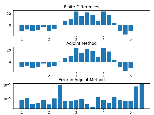
Verification of gradient accuracy.

This shows the individual derivatives computed using finite differences and the adjoint method and computes the relative error in each derivative (with respect to the finite difference).

Whenever we setup an optimization it is essential that we verify that the gradients are accurate as we have done here. If the gradients are not accurate (error \(> \sim 10^{-2}\)), then we are significantly more likely to run into issues during the optimization. Once we have verified their accuracy, we can continue on to running the optimization with high confidence that the optimization will “work.”

Note

What do we mean by gradient accuracy in this case? In EMopt, the gradient calculated using the adjoint method is compared to a gradient calculated using brute force finite differences. Given these two gradients \(\nabla_\mathrm{FD} F\) and \(\nabla_\mathrm{AM} F\), the error is defined as

error = \(\frac{\bigg|\nabla_\mathrm{FD} F \cdot \nabla_\mathrm{AM} F\bigg|}{\bigg|\nabla_\mathrm{FD} F\bigg|}\)

4.5. Running the Optimization

In the previous sections, we have setup the grating coupler simulation, defined a parameterization, defined a figure of merit, and verified that our gradients are being computed correctly. The only thing left to do is to setup and run the optimization!

Setting up an optimization is straightforward with the help of the Optimizer class. This class provides an interface to the scipy.optimize.minimize() function. The process for setting up the optimizer is as follows. In PART 12 we write:

fom_list = []
callback = lambda x : plot_update(x, fom_list, sim, am)

# setup and run the optimization!
opt = emopt.optimizer.Optimizer(am, design_params, tol=1e-5,
                                callback_func=callback,
                                opt_method='BFGS',
                                Nmax=40)

# Run the optimization
final_fom, final_params = opt.run()

This sets up an Optimizer object which takes our AdjointMethodPNF object, and initial guess for our design parameters, and a number of other optional arguments. Calling opt.run() runs the optimization using the BFGS algorithm as we specified using the opt_method argument.

You will notice that another one of the optional arguments that we passed in was the callback_func parameter. This allows us to pass a function to the optimizer which it will then call at the end of each iteration of the optimization. In this case, we define a callback function called plot_update() (PART 13):

def plot_update(params, fom_list, sim, am):
    print('Finished iteration %d' % (len(fom_list)+1))
    current_fom = -1*am.calc_fom(sim, params)
    fom_list.append(current_fom)

    Ez, Hx, Hy = sim.saved_fields[1]
    eps = sim.eps.get_values_in(sim.field_domains[1])

    foms = {'Insertion Loss' : fom_list}
    emopt.io.plot_iteration(np.flipud(Ez.real), np.flipud(eps.real), sim.Wreal,
                            sim.Hreal, foms, fname='current_result.pdf',
                            dark=False)

    data = {}
    data['Ez'] = Ez
    data['Hx'] = Hx
    data['Hy'] = Hy
    data['eps'] = eps
    data['params'] = params
    data['foms'] = fom_list

    i = len(fom_list)
    fname = 'data/gc_opt_results'
    emopt.io.save_results(fname, data)

This function prints out the current iteration number, generates a plot of the current state of the optimization (figure of merit, fields, and structure) and then saves the current state of the optimization to a file. In order to save a plot of the state of the optimization, the io.plot_iteration() function is a convenient option. Alternatively, you may generate your own plot using, for example, matplotlib. In order to save the data file, we use the io.save_results() function. This function takes a file name (without extension) and two dictionaries containing any data you would like saved. The first (required) dict may only contain particular “identifiable” data like the field arrays, permittivity array, figure of merit, etc. An additional dict with arbitrary contents can be supplied and saved as well (using the optional additional argument). This function saves the contents to the widely recognized hdf5 format.

It is important to note that the plot_update() function takes multiple arguments however the Optimizer class expects a function with only one argument (the design parameter array). In order to get around this, you will note that we defined a lambda function that effectively hides away the additional arguments. This is the easy and effective solution.

If everything is setup correctly, the optimization should complete after 27 iterations. This process takes around 37 minutes on an Intel Xeon E5-2697 v3. The final fields, structure, figure of merit history should look something like this:

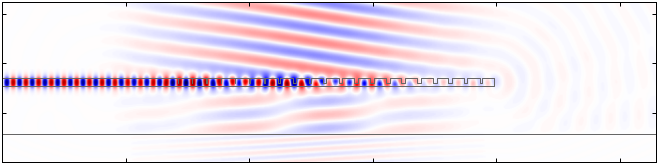
Simulated fields of the optimized grating coupler.

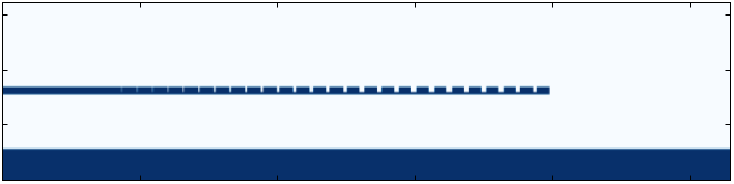
Permittivity distribution of the optimized grating coupler.

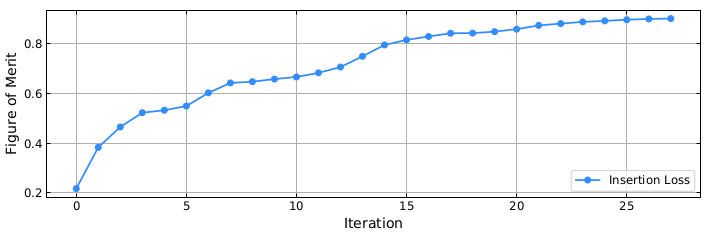
Progress of the figure of merit during the optimization.

Congratulations! You have optimized a grating coupler! This optimized grating achieves a very high coupling efficiency of 90% (-0.45 dB) and gives you a sense of what we can achieve using EMopt!

4.6. Taking Things to the Next Level: Constrained Optimization

If you look at the final result of our optimization, you will notice that the optimized structure contains some very small features. In reality, these features will not be resolved using deep UV lithography. In order to account for this, we can run a constrained optimization.

The basic process for running the constrained optimization is very similar to the optimization we just put together. There are three main differences:

1. We use the previous result as the starting point instead of a simpler physically-intuited structure.
2. We parameterize the grating in terms of the actual slot widths and periods.
3. We impose an additional penalty term to the figure of merit which reduces the figure of merit if slots in the grating become too narrow.

To see how all of this is done, check out the gc_opt_constrained.py example file.

4.7. References

[1] Andrew Michaels and Eli Yablonovitch, “Inverse design of near unity efficiency perfectly vertical grating couplers,” Opt. Express 26, 4766-4779 (2018)

[2] Andrew Michaels and Eli Yablonovitch, “Leveraging continuous material averaging for inverse electromagnetic design,” Opt. Express 26, 31717-31737 (2018)